Deep learning models can produce state of the art performance for malware detection, but that performance comes at a price: memory intensive models with slow processing times. A lot of research (see, e.g. “The Lottery Ticket Hypothesis” , or “Optimal Brain Damage” ) has suggested that the large parameter space of deep learning models is mostly useful during training. Once the model has been fully trained, many of the parameters are either unneeded or redundant, and can be removed.
In this post, we’ll explore a few of the methods that have been proposed for training smaller models, and see what happens when we apply them to a malware detection model.
Trimming connections vs trimming nodes
In their most basic form — and the form we use for malware detection models — deep learning models are a long series of alternating between matrix multiplications and activation functions. If we have a minibatch of k samples with n features, a hidden layer with m units, and an activation function f , then the computation for the first layer looks like this (with array dimensions in the subscripts):

Where b is a (1 × m) vector that gets replicated k times. The majority of the parameters are in the layer weights, W, which we are trying to prune. The simplest way to prune W is to set individual entries to a value of 0 — this makes the matrix sparser and more compressible, but in most cases requires the same amount of memory and almost the same number of computations during inference.
The more drastic way to prune W is to remove entire nodes from the network rather than just individual weights — essentially deleting entire rows or columns. This is a much more drastic change to the network, which has a much greater impact to affect accuracy, but can also lead to significantly smaller and faster models.

How to (safely) trim your brain
The main idea underlying almost all network pruning approaches is simply to remove the “least important” weights or units from the network over time, while trying to balance the degree of pruning with the accuracy of the final model. The way that importance is measured tends to fall into three main groups[i]:
- Directly equating magnitude of the weight (or the magnitude of the change of a weight during training) with importance (see, e.g. “Learning both Weights and Connections for Efficient Neural Networks” or the Lottery Ticket Hypothesis): the smallest (in absolute value) weights are trimmed first. While this is less sophisticated than other approaches, it frequently leads to excellent results, especially if combined with a retraining or fine-tuning step.
- “Optimal brain damage”(or OBD) and related methods, which looks at the second derivative of the weights with respect to loss. Rather than assuming that smaller weights will have less contribution, this approach looks at the sensitivity of the loss function to the parameter, and removes the ones that are least sensitive first.
- Online methods, that try to learn importance (and remove unimportant elements) in the process of training (see, e.g. “Learning Sparse Neural Networks through L0 Regularization”, “Targeted Dropout”, or “Smallify: Learning Network Size while Training”). Depending on how you like to think of it you could either view this as a form of regularization or as a way to combine model selection/pruning and model fitting into a single step.
To avoid the potential complexity of retraining, we implemented three of the online methods and compared them to a “baseline” malware detection model (our ALOHA model). We used 9,000,000 samples to train the model, and tested on 1,000,000, and trained each model for 20 epochs.
The Smallify and Targeted Dropout (Node-TD) methods both targeted nodes, while the L0 regularization method targeted individual weights. The performance of the models is plotted below as overlaid ROC curves. All three compression methods produced roughly comparable results up to the lowest false positive rates, at which point Targeted Dropout began to lag in performance.

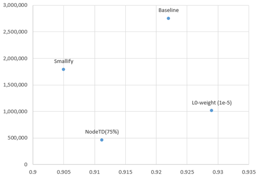
If we look at the degree of size reduction, we can further explore the trade-off. On the plot below the x-axis is accuracy at a false positive rate of 1 in 1000 — which is about where we deploy most models — and the y axis is the total number of parameters in the model. While Node-TD gives us the best overall reduction in size at 17% of the original number of parameters, it does so at a slight cost to performance. The L0 method — which again targets weights — doesn’t give as much of a parameter savings (since it’s removing individual weights, not entire rows/columns) but actually slightly improves overall performance of the model while still reducing the total size to about 37% of the original number of weights!

Conclusion
When it comes time to deploy models, size as well as performance can be potential issues. By taking some tricks from the existing literature on model pruning, it’s possible to significantly reduce the size of models while at the same time not significantly harming overall performance. Keep an eye out for our next post on this topic where we cover offline methods of pruning, and look at combining them with online methods!
Rich Harang is Research Director for the Sophos AI team; find him on twitter at @rharang
[i] Careful readers might notice an apparent omission from this list: there are “zeroth-order” methods (trim based on weights) and “second-order” methods (trim based on an approximation of the Hessian), but no “first-order” methods (trim based on the gradient). The main reason for this is that most trimming is assumed to happen when the model is fully trained, at which point the gradients of the parameters are all — either in practice or by assumption — approximately zero.