Introduction
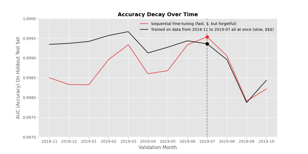
In the last blog post (linked here for anyone who missed it), I explained what catastrophic forgetting is and why we want to avoid it. Essentially, if we can get a sequentially fine-tuned deep neural network model to match or beat the accuracy of the same deep neural network model trained all at once, then we have a path to deploying accurate models very quickly and very cheaply. This blog post will dive into some methods we tried, and will be much more technical.
Methods & Results
Model Averaging
What did we try out? First, some methods that failed. Negative results are still results!
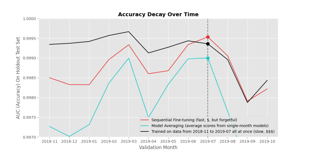
What if you train separate models on each month, and then just average the scores of your monthly models? Well, see in Figure 2 that this did worse than either of our base methods (red and black), which made me happy, because I didn’t want to have to handle productionizing a bunch of ensemble models.
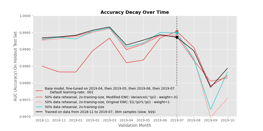
Data Rehearsal
OK, now onto something more successful. A common method of avoiding catastrophic forgetting is called data rehearsal. Data rehearsal just means mixing in some old data with the new data during fine-tuning. It works really well, but it does mean you need to maintain access to your older data (or at least an iid (independent and identically distributed, i.e. random) subsample of it), which isn’t always possible.
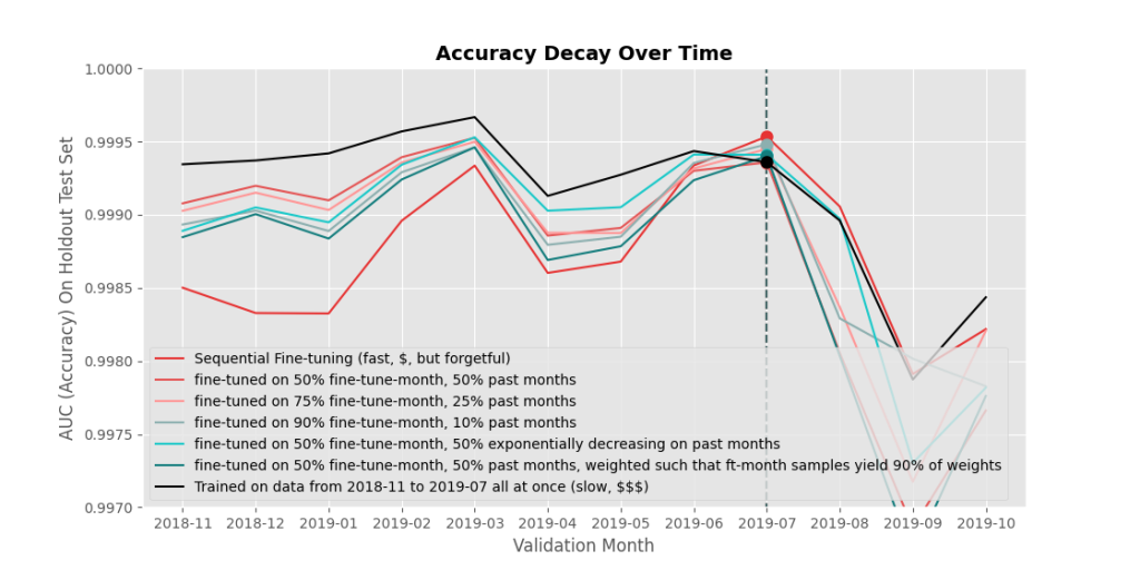
Mixing in old data also increases the amount of training data you have, so it takes longer to train the model one epoch. In order to make method comparisons more equal, when testing out data rehearsal I fixed the fine-tuning epoch sizes to 4 million, and adjusted what proportions came from past data. 50% seemed to work well in my experiments. If you’re willing to not fix the fine-tuning epoch size (i.e. allow it to increase with added past data), you can get even better results, shown at the end of this post.
Looking at the results in Figure 3, mixing in old data improves the forgetting effect, but doesn’t eliminate it, while the accuracy on future data is also diminished. What about some other methods?
Regularization
If you can’t just mix in old data, the next logical option is to suppress the movement of parameters, to limit ‘forgetting’. You can do this naively, like via $L2$ regularization, or by reducing your model’s learning rate. This can help forgetting-effects quite a bit (at the maximum, no parameters are changed, so there’s zero forgetting), but can also hinder learning new content (again, at the maximum, zero parameters are changed, so there’s zero additional learning).
Figure 4 shows $L_2$ regularization: an $L_2$ loss penalty is added to each parameter with respect to the current parameter’s value $\theta_{c}$ during fine-tuning, and the previous model’s parameter value $\theta_{p}$. The further away you move from the previous model’s parameter value, the higher the penalty:$(\theta_{c} – \theta_{p})^2 $.
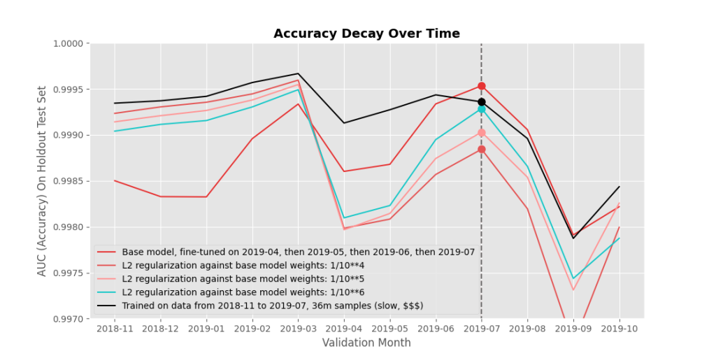
As expected, forgetting is reduced but learning is reduced too. There’s a very clear tradeoff, and I’m not particularly convinced that it’s worth it to apply $L_2$ regularization. Interestingly, though, we got different results when adjusting the learning rate. Adjusting the learning rate forces smaller step-sizes to be taken, which – generally speaking – slows down learning, risks getting stuck in local minima, and risks overfitting (risks getting ‘too deep’ in a local minima).
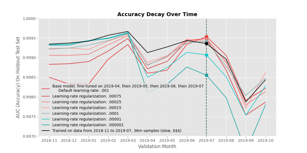
Here, lowering the learning rate during fine tuning almost universally shifted accuracy towards the black line (our goal)! If the learning rate is really low (dark turquoise), forgetting is minimized but learning the fine-tuned months is greatly reduced, similar to $L_2$ regularization. But check out the model with a learning-rate of $.0001$ (a tenth of our default value) – that grey line is almost universally closer to our goal (black line) compared to the default fine-tuning approach (red line). That’s… surprising. In fact, does it even make much sense that reducing the learning rate uniformly would help catastrophic forgetting?
I buy that it forgets things more slowly, because learning is slower, and perhaps it’s finding local minima that a larger learning rate would skip over, but it felt like something else was going on.
I think it’s likely that our model in general is able to find a better (more delicate) local minima when the later stages of training are done with a lower learning rate (parameters move in smaller step sizes), and that benefit comes through in the results. To verify this, I took the retrained model (black line) snapshot of a few epochs before it was finishing training, and finished training it with a learning rate of $.0001$ in those last few epochs. I found that the resulting test accuracy on all training months increased universally.
So adjusting the learning rate helped, but that seems to me more like a happy accident as opposed to a clever trick to reduce forgetting. Lowering the learning rate or applying $L_2$ regularization is basically telling the model to suppress all parameter movements, regardless of the parameter, during fine tuning. That can’t be ideal! What about more intelligent forms of regularization?
Regularization – Elastic Weight Consolidation
What if we could let the model change parameters that don’t matter so much for classifying older data, more heavily penalizing changes to others? Elastic Weight Consolidation (EWC) is a method developed by researchers at Deep Mind in 2017 that attempts to do just this. The idea is to think about your base model as a Bayesian prior of the parameter estimates – then fine tuning is just applying more data to approximate the posterior. Essentially, you apply regularization that simulates the prior distribution. EWC assumes that the prior is normally distributed: with mean given by the base model’s parameters, and variance given by the inverse of the Fisher Information matrix diagonal $F$.
Instead of minimizing loss during fine-tuning with respect to your new training data, you minimize an estimate of your loss with respect to both your past $p$ and current $c$ data:
\[ L_{p,c}(\theta) = L_{c}(\theta) + \lambda L_{p}(\theta) ≈ L_{c}(\theta) + \sum_i^{n}{\frac{\lambda}{2} *F_{i, p} * (\theta_{i, c} – \theta_{i, p})^2 } \]
So what we have here is $L2$ regularization, scaled by a scaling parameter $\frac{\lambda}{2}$ and by this $F_i$ value for each parameter $\theta_i$.
The next section will get into the math behind this formula, but it’s totally skippable if you’re not feeling mathy today.
Regularization – Elastic Weight Consolidation – Some Mathy Bits
The particularities of the formula appear to come from using Taylor Series / Laplace Approximation. Loss with current parameters on current data (fine-tuning data) is known, but estimating loss with current parameters on past data is not known. Without access to past data during fine-tuning, but with access to saved partial derivatives of loss on past data with previous parameters $\theta_{p}$, you can estimate the loss $L_p$ on past data with current parameters $\theta_{c}$ via Taylor Series:
\[ L_p(\theta_{c}) = L_p(\theta_{p}) + \frac{\partial L_p}{\partial \theta_p}(\theta_c – \theta_p) + \frac{1}{2} \frac{\partial^2 L_p}{\partial \theta_p^2}(\theta_c – \theta_p)^2 + … \]
Because we’re minimizing loss through gradient descent, we only care about terms that aren’t constant with respect to $\theta_c$. So the first term on the right hand side of of the equation we can drop. The second term we can assume is 0 because $L_p$ was at a local minimum with previous parameters $\theta_p$ (before fine-tuning), and the fourth term ($…$) we’re choosing to drop as “small change”. What we really want to estimate is the loss of both current and previous data on current parameters $\theta_c$, so adding $ L_c(\theta_{c})$ to both sides of our equation leads us to:
\[ L_{p,c}(\theta_c) = L_c(\theta_{c}) + \frac{1}{2} \frac{\partial^2 L_p}{\partial \theta_p^2}(\theta_c – \theta_p)^2 + constant \]
Replacing $\frac{1}{2}$ with the scaling term $\frac{\lambda}{2}$, leads us to an equation that looks very similar to the one the EWC paper shows.
If you’re still with me, you might be a little flummoxed. The formula we arrived represents fisher information $F$ as $\frac{\partial^2 L_p}{\partial \theta_p^2}$. But is that what Fisher Information is?
Well, with your model’s (negative log likelihood) loss as $L_p$, the Fisher diagonal is defined as $E(-\frac{\partial L_p}{\partial \theta} * -\frac{\partial L_p}{\partial \theta})=E(\frac{\partial L_p}{\partial \theta} * \frac{\partial L_p}{\partial \theta})$ – the negatives coming from the ‘negative’ log likelihood and then cancelling out. (It’s interesting to note that when loss is at a local minimum and thus $E(\frac{\partial L_p}{\partial \theta})=0$, $E(\frac{\partial L_p}{\partial \theta} * \frac{\partial L_p}{\partial \theta})$ is the same as the $variance(\frac{\partial L_p}{\partial \theta})$).
Under certain regularity constraints (which don’t hold true, but meh), the Fisher diagonal value is equal to the negative expected second partial derivative of the Loss $L$ with respect to $\theta$: $- E(-\frac{\partial^2L}{\partial \theta^2}) = E(\frac{\partial^2L}{\partial \theta^2})$ – i.e., the diagonal of the Hessian of the negative log-likelihood (loss) with respect to parameters: i.e., what we had in our derivation formula!
A more intuitive way to think about this is that $variance(\frac{\partial L}{\partial \theta})$ might be a nice way to estimate how sensitive your model is to changes in $\theta$. When loss is greatly affected by small changes to a given parameter $\theta_i$ (i.e. $variance(\frac{\partial L}{\partial \theta_i})$) is high), then the `confidence’ that $\theta_i$ should not be changed is high, so the variance in the prior distribution should be small (tight). The added regularization term simulates this confidence, so that parameters the model is very sensitive to don’t end up being changed much.
While the derivation uses one form of Fisher Information,
in practice, I think you have to use the $E(\frac{\partial L}{\partial \theta} * \frac{\partial L}{\partial \theta})$ version on deep neural networks. Can you guess why?
If, for any parameter $i$, your $F_{i,p}$ term is less than zero, then the resulting regularization term will actually just keep on pushing $\theta_i$ further and further away from $\theta_{i,p}$ (the previous value), which will tend to wreck any model. The $E(\frac{\partial L}{\partial \theta} * \frac{\partial L}{\partial \theta})$ form of fisher $F$ is guaranteed to be positive, while the $E(\frac{\partial^2L}{\partial \theta^2})$ form, not so much. In practice, we found that about a third of our $E(\frac{\partial^2L}{\partial \theta^2})$ estimates tended to be negative, causing very poor results.
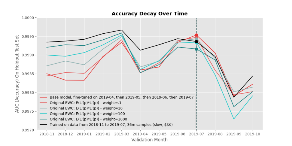
Figure 6 shows results from EWC, using the $E(\frac{\partial L}{\partial \theta} * \frac{\partial L}{\partial \theta})$ formulation of $F$. The results look… okay? I was expecting better, given that the results in the paper look great. But a big difference between the models we tend to work on at Sophos and the models in a lot of machine learning papers, is that ours our much bigger, trained on much more data, and thus their loss functions are much more complicated than ones often used in papers. As a result, I wonder if the many assumptions EWC makes end up messing up the estimate by quite a large amount.
Conclusion
In the end, by far the most effective strategy I found for avoiding forgetting is to just mix in a little of your past data with your current (even if you only have access to a partial sample of your past data). Doubling your fine-tuning training size and sacrificing half of that to rehearse past data achieves about the same results as retraining everything from scratch, while only upping training time by a factor of 2, as opposed to a factor of, say, ten or more, depending on how far back your data goes. Figure 7 shows the results of data rehearsal combined with our various regularization techniques, and I can’t say one really beats just using data rehearsal alone.
Thanks for reading!