
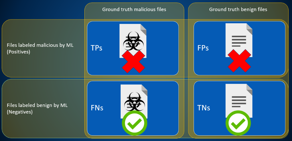
Introduction
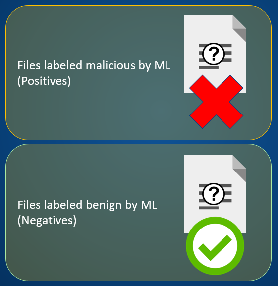
When we move machine learning models from the lab to the real world, tracking and evaluating model performance becomes a lot harder. Rather than having a set of data where every sample has a label and we can immediately answer the question “did the model get it right?” we have a huge volume of data where we don’t know any of the labels, only what the model said about it. To make matters worse (at least from the perspective of evaluating the model) the data is overwhelmingly biased towards benign files; if we wanted to try to find malware that our model missed, we’d have to manually analyze thousands of files to find a single example.
While we can estimate the model false negative rate from our training data (if we’re willing to assume that our training malware looks like real world malware), that doesn’t help us estimate the number of malware samples we should have caught. Knowing we catch 90% of all malware doesn’t help us answer the question of “how many malware samples did we miss?” unless we know what the rate of malware in our customer data is. If there are 1,000 malware samples in some telemetry sample, then we probably missed somewhere around 100. If there are 100,000 malware samples in some batch of telemetry, we probably missed 10,000.
What we really need is an estimate of the overall rate of occurrence of malware in our training data: an answer to the question “Out of every 100,000 samples, how many of them do we expect to be malware?” We call this number the “base rate” and, while it’s surprisingly hard to estimate in practice, once we do so, it provides us the key to unlock a complete evaluation of our model’s performance in the wild.
An epidemiology analogy
While the domains have significant differences, in some respects, the way we must rely on (imperfect) tests to learn about the prevalence of malware mimics the kinds of problems epidemiologists face when tackling epidemiological question: we might know the total number of people in a city, as well as how many we tested for some disease and the number of those people who ultimately tested positive, but how do we go back to estimate a total infection rate for the entire population? Say, just for the sake of an example, that we tested 35,000 people and got 2,029 positive results from a test know to have a detection rate of 95% and a false positive rate of 3%. If we have 140,000 people in our city, how many people in the city are likely to be infected?
It’s not as simple as taking the positive rate of the tests and extrapolating that to the total number of people. There are two issues with that approach:
- The tests have an error rate: some people who don’t have the disease will get positive tests in error, and some people who do have it will be told that they don’t.
- This is fundamentally a statistical problem: the part of the population that you tested is a sample – with sampling error – and the true/false positive results are also probabilistic in nature.
But despite these challenges, we might want to try to figure out what the actual rate of infection across the population of the city is, and put confidence intervals around our guesses.
So, what can we do?
Imagine, for a moment, that we have access to a time machine and a parallel universe generator (bear with me!) that will let us travel back in time one week and branch our universe at that point into millions of other universes where our generator lets us set the infection rate by hand. If we did that – for a range of infection rates – and then waited a week, we could peek into all those universes and see which ones had results that closely matched ours. We then go back and look at the infection rate that we set for those universes that look most like our own, and take those infection rates as ‘good guesses’ for the infection rates in our own universe. There will naturally be some spread of rates, and we can take that spread as an indication of the distribution of possible rates that might have resulted in the test results we saw from our real/original universe.
Unfortunately, time machines and parallel universe generators are still hard to come by, so if we’re willing to make some simplifying assumptions, we can turn to simulation, as shown in the python code below. We provide a proposed infection rate and the number of tests that were performed as an input, add information about the true and false positive rate of the test, and then from there a short function simulates the number of positive results we’d get from that test.
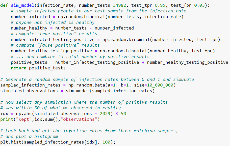
The code above is essentially going through the same exercise, shown schematically below. We pick an infection rate, and then simulate the number of positive results we’d see given that infection rate. Whenever that number of positive results “close enough” to the number of positive results that we observed, we keep the infection rate that generated that sample, and then build up a histogram of possible infection rates, generating a distribution such as the one on the right in the figure below.
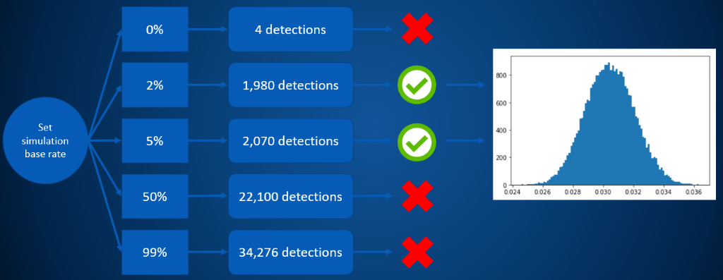
So in this example, we can estimate that the most probable infection rate is somewhere in the ballpark of 3.04%, but also that numbers as low as 2.74% or 3.36% are also quite plausible, if less likely.
If we stop and think about what this estimate for the infection rate is telling us about the number of infected people in our sample, we see some interesting math fall out: a 3.04% infection rate implies about 1,065 infected and 33,917 healthy individuals within the sample that got tested. If we use the 95% detection rate, that gets us 1,065×0.95≈1012 true positives, and the 3% false positive rate gets us 33,917×0.03≈1018 false positives. But if that’s right, then we’re saying that over half of our 2029 positive test results are in fact errors, our model precision is less than 50%!
This is exactly what is meant when we discuss the problem of a base rate. Because the number of infected people is overwhelmed by the number of uninfected people, even a modest false positive rate means that many – if not most – of your positive test results will actually be errors.

What about malware?
In the case of infectious diseases, we’re looking for a single disease, and have a fairly good idea of the accuracy of the diagnostic test. When we move from our infectious disease analogy to the case of malware, we’ve got an extra problem to solve before we can apply the same sort of analysis as above: getting a good estimate of the model’s accuracy. A lot of factors contribute to the uncertainty in these estimates. We retrain our model regularly, and the kinds of malware that are out and about causing trouble in the world also change over time. Both factors mean that the model True positive rate (TPR) and False positive rate (FPR) will change over time, and so we need to estimate that as well. Fortunately, we have an overlap between some files we have labels for and files coming in from our customer telemetry. This lets us estimate our true and false positive rates, at least up to a degree of accuracy (for the technically inclined: check out the endnotes for details on how exactly this happens[1]) and feed samples from those distributions into our estimation as well. Some example estimates from our data (May of 2020) showing the estimated true and false positive rates of our model at the deployment threshold are shown below.
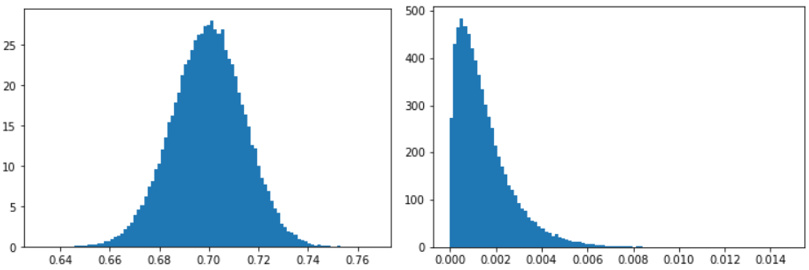
This adds a bit more complexity to our modeling, but not much. Rather than taking our model TPR and FPR as fixed and known, we now sample those as well based on the labeled data. As you can see, due to the limited sample size, we can’t be extremely precise about the actual rates, however we can still narrow them down to usable ranges. And, crucially, this uncertainty will propagate correctly into our base rate estimates!
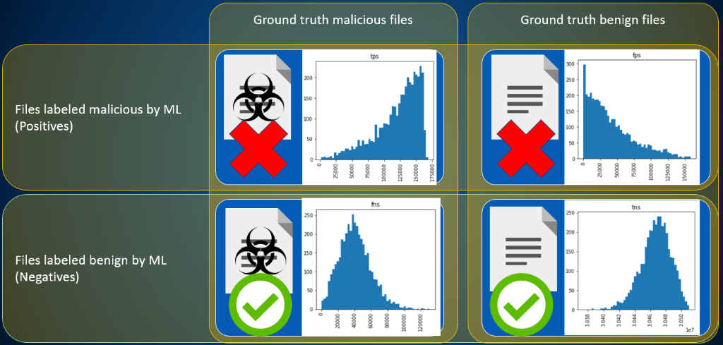
The simulation itself simply takes model true and false positive rates as well as base malware rate, and returns the plausible samples to us; however in the process of simulating the detection count (which is what we use to filter our samples), we also have to simulate counts of the model true and false negatives and positives. We can retain these samples as well, and use them to gain direct insight into what is likely happening with our model for a particular evaluation period. Below we show a set of those samples for a week in May of 2020, highlighting that – while the analysis is somewhat uncertain about the exact distribution of true and false positives – the true positives are likely concentrated close to (but not exactly at) the number of positive detections for the week, and the false positives are heavily skewed towards zero. The distribution of malware that the ML model missed – because we set our detection threshold so high to mitigate the base rate problem – is concentrated around a value of approximately 40,000, and of course true negatives dominate the overall distribution.
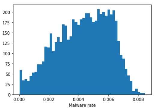
Finally, obtaining the base rate is straightforward. In each simulation that we kept (again, as having a final result that was close to the result we saw in reality) we know the number of true positives and false negatives we saw in the course of the simulation. Combining these gives us the total number of malicious samples from each simulation, which we can divide by the total number of samples to obtain the final malware rate from each simulation. When we plot the density of those results, we can get an estimate of the total amount of malware in customer telemetry from that time period, in this case we can estimate a 95% confidence interval of 0.06% to 0.6% malware in our customer telemetry, with a median estimate of 0.4%.
Conclusion
By using a simulation-based model, which takes some inspiration from epidemiological modeling, we can generate principled, Bayesian estimates that capture the “dark matter” of model evaluations in the field: not just statistics on what we detected, but also estimates of what we missed. While these estimates won’t tell us which particular samples we made mistakes on, being able to estimate the model’s performance when it returns a verdict of “benign” gives us the complete picture of how our model is actually performing in the real world under the deployment conditions we have selected.
Postscript
It bears mentioning here that this evaluation only covers the ML component of our endpoint security solution, which is just one component of a much more complete technology stack that encompasses a much wider range of technologies to both detect things that ML misses and to compensate for errors that the ML tends to make.
Endnotes
[1] We treat our TPR/FPR/TNR/FNR as coming from a probability simplex and apply a Dirichlet/Multinomial model to it by taking the counts of TPs, FPs, TNs, and FNs where we have an overlap between telemetry and labeled data as samples from a multinomial parameterized by the unknown rates; this posterior estimate of the probability vector is what we use when sampling model TPR and FPR. We set the prior for malware base rate to Uniform distribution on the interval (0,1).