
Introduction
On any given day that we are happily browsing the Web, we are stomping around on a minefield. Malware is lurking under the surface. Clicking on an infected link can result in malicious programs being downloaded to your device and taking control of your data, or it can attempt to persuade you to provide sensitive personal information on a bogus website for attackers to collect and use to impersonate you. These bogus websites are often crafted by attackers to replicate the look and feel of well-known, trusted, safe websites. The goal is to exploit human gullibility and deceive users tricking them into sharing login credentials, credit card numbers, and other personal information. Such malicious practices that rely on social engineering are commonly referred to as phishing. According to the FBI’s 2020 Internet Crime Report, phishing was the top 1 cybercrime of 2020 based on victims’ reports [1]. For this reason, one should tread carefully and avoid clicking on malicious URLs that point to compromised Web resources.
Take a look at the following URLs:
- http:\\1stopmoney.com\paypal-login-secure\websc.php
- http:\\31.14.136.202\secure.apple.id.login\Apple\login.php
How much do such links tingle your Spidey senses?
To the trained eye, these links immediately stand out as at least highly suspicious, and almost surely malicious. So we asked ourselves: can a machine learning model be trained to do the same task: gauge the maliciousness of a URL simply given the URL itself?
Our short answer is yes, definitely; we built it. Our model takes in a raw URL string as input and classifies it as malicious or benign using nothing but the URL itself to make a decision: no need for additional information about the content of the webpage itself or about the network. Just the URL (we provide a quick demo here). At the time we developed this model (back in 2017), it was the first of its kind in the cybersecurity literature to solve this detection problem given so little information.
The question “But how does this model do that task?” takes a bit more explanation.
The building blocks for learning about URLs
The model is made up of three main modules working together. Each one performs a relatively simple task, then hands its results to the next module, allowing the final module to make a decision about the URL.
- Character embedding
- Feature detection/extraction
- Classification
Let’s dive into the details of each one:
Step 1: Character Embedding
URLs, when you break them down, are just strings of letters, numbers, and some special characters (like the slash “/”). Machine learning models like to work with numbers, though, so the first challenge in building a machine learning model for URLs is to turn the string of a URL (like “hxxp://paypal.com”) into some sort of numerical format ([1.1, 12.3, -4, …]). To do this, we use something called “embeddings”: where we represent each character with a list of numbers, and then build a “list of lists of numbers” (technically: a “matrix”) to represent the whole URL. This matrix is basically a list with one embedding (read: list of numbers) for each character of the URL. You can see an example of this in figure 1, below, where we have some number (call it $s$) of letters in the URL, and we’ve decided that each embedding list will be some number (say, $m$) of values long (you might see this number $m$ — whatever we decide to set it to when we start building the model — called the “embedding dimension” in some places). Notice that every time a ‘w’ appears it has the same embedding as every other ‘w’ in the URL, and similarly for the ‘u’, ‘s’, and so on. We substitute that letter’s embedding into the matrix no matter where in the URL that letter appears.
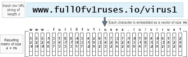
If that all seemed a bit heavy, don’t worry too much about it. The big idea is that we turn individual letters into lists of numbers (or “embeddings”), in a way that helps it tell good URLs from bad ones.
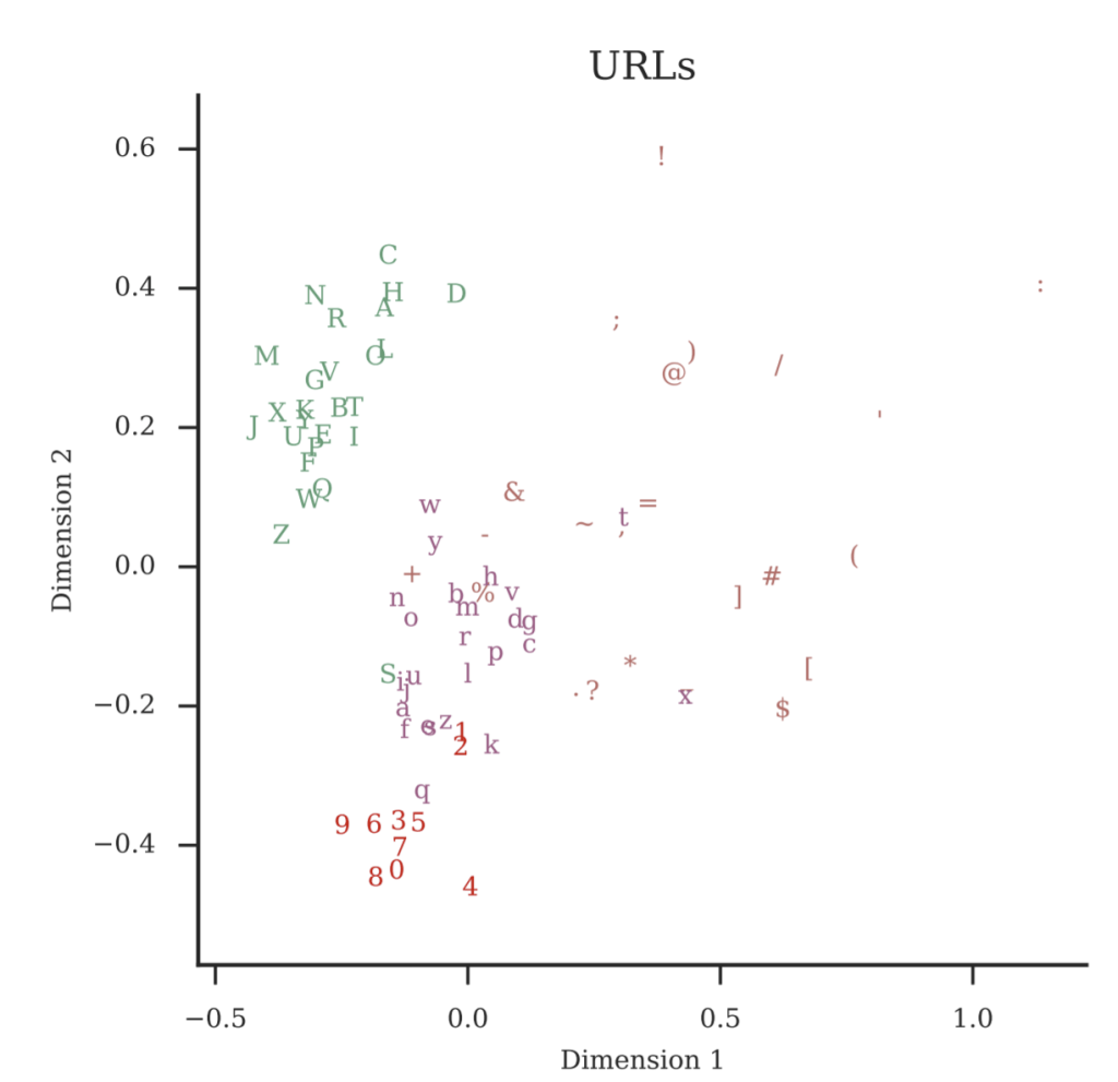
But that leaves the question: what should those embeddings be? What exact numbers should we use? Surprisingly enough, we can just start with random embeddings and let the model “figure out” what the embeddings should be as part of learning to detect bad URLs. If you show the model enough URLs, eventually it can figure out for itself how to represent characters that have similar roles in a URL with similar embeddings for those characters. You can see this in figure 2: we’ve taken the embeddings that the model has learned after training from all our characters and represented them in two dimensions. As you can see, a lot of the capital letters end up in the same region, numbers group together, and lower-case letters are all clustered. On its own, the model has learned something about the space of characters in a URL: which ones are most like each other, and which ones might have a special function. Crucially, we didn’t have to tell the model about this, it can figure it out directly from the data.
For our model, we set the length of the URL input to $s=200$ and the length of each character embedding (the embedding dimension) to $m=32$. Since our model deals specifically with URLs and only 87 distinct agreed upon characters can be used to make a URL string, we define the embedding vocabulary (the unique characters that the model can expect to encounter and embed) to be those 87 characters.
But what happens if the URL is shorter or longer than 200 characters? That’s actually one of the easiest parts:
- If the input URL string is longer than 200 characters, simply cut off characters from the beginning of the string.
- If it is shorter than 200 characters, add a special null character to the front as many times as needed to get to the limit of 200 (this is usually referred to as padding).
Note: In practice, we have made some slight changes to our model throughout the years. Currently we pad and truncate at the end of the URL string to conform to the 200-character length. The above two rules were however what we used to obtain our original model for which we present the experimental setup and results in this blogpost.
Step 2: Feature Extraction
So far, we have worked out a way to convert a URL string to a numerical representation with embeddings –something the subsequent parts of the model can work with. Now we can start extracting useful information from it to be able to make an informed decision regarding the maliciousness of the original input URL. For this purpose, we use a convolutional neural network (CNN or ConvNet). Even though they were originally developed to deal with classifying images, CNNs can be adapted to solve numerous tasks, including string classification. Given an input matrix (our “embedded string”, this network will progressively detect patterns and relevant clues (in the literature, these patterns are called “features”) then use them to decide how probable it is that the input we gave it belongs to one class or another: in our case “benign” vs. “malicious”. This ability to automatically learn to spot useful evidence from the input (what we call feature extraction) is precisely why we don’t need to craft any additional features ourselves and can afford to give only the model only the raw URL string, and then sit back and relax as the model learns to tell good from bad, benign from malicious.
So this is awesome stuff! But how are ConvNets able to do this?
A brief digression: Convolutions and images
As mentioned earlier, CNNs were initially developed to deal with images, and what is an image but a matrix of pixel values — rows and columns of numbers. For instance, a grayscale (black-and-white) image can be represented by only one matrix of pixel values ranging from 0 to 255 capturing how “light” that pixel is, with 0 for black and 255 for white and in-between are shades of grey. When you have a color image on the other hand, it can be represented by 3 matrices on top of each other with each one corresponding to a color: either red, green, or blue (RGB). Each one has values between 0 and 255 for the different shades of that color. By putting the 3 matrices together, you can get any color you want, kind of like when you mix colors to paint: blue + red = purple.
Another important thing with images is that more often than not, pixels that are close to each other tend to have similar values and convey more meaning together than if taken individually (think of a patch of blue sky in an image, or a red flower for instance). A CNN takes advantage of this property: when trying to look for patterns in the input, it looks over a group of pixels at once using “convolutional kernels” (aka. filters) — small square matrices holding special numbers called “parameters”. What is so special about these numbers?
Each convolutional filter acts like a detective. It goes around and asks questions to gather evidence. Each filter asks a specific question through the values of its parameters. At first, a CNN asks simple questions: “is there an edge?”, “is there a lot of red?”, and as its investigation advances, it asks more complex ones “is this a red flower?”. Eventually, the model learns to ask better questions, whose answers lead it to correctly figuring out the class of the input (“rose” as opposed to “pineapple” for instance). Better questions are expressed through adjusting those parameters we were talking about. Mathematically speaking, “asking a question” is performing a dot product between the filter’s parameters and a region of the image matrix.
When looking for answers, a filter needs to search all over the image since relevant clues can appear anywhere. For this reason, each detective matrix -convolutional filter- slides over the entire image across width and height. This operation results in the production of “activation maps” (aka. feature maps) which can be considered as reports that each filter gives. Each map basically summarizes which parts of the image answer a corresponding filter’s question and to what extent. These maps are stacked together and more filters may be applied to them in order to piece the clues together to get closer to solving the classification task.
This sliding the filter over the input, coupled with dot product computations, is what is referred to as a “convolution”. Figure 3 provides a visualization of a convolution. Note that in practice there is no sliding per se, but that’s okay since whatever cool points the network implementation loses due to the lack thereof, it largely compensates for in parameter sharing. Instead of the same filter sliding and going over the entire image, copies of the same filter (i.e. filters that share the same parameters) go to different parts of the image to produce one activation map. The parts of the model that are in charge of applying convolutions and figuring out progressively better filters are called convolutional layers.
Convolutions for text
Now let’s go back to detecting malicious URLs. Instead of an image matrix, we simply use the URL matrix we obtained by embedding the original input string. With the URL matrix as input, our ConvNet follows the same logic as described previously. It just does that investigative process four times since we use four convolutional layers in parallel. Every single one of them is armed with 256 filters that slide over the URL matrix to gather all the needed intel (i.e. detect relevant features). Each layer also specializes in applying filters of a specific size. We use filters with 2, 3, 4, and 5 numbers respectively to detect various patterns and subsequences within the URL. Then we take the resulting activation maps from each one of the four layers and add them up respectively; this operation is SumPool. We do this in order to summarize the degree to which relevant patterns (for each layer) occur in the URL. After that, we concatenate them together to obtain a concise list of 1,024 numbers representing the results of our inquiry.
Classification
Armed with those answers, we can start piecing everything together to classify the input. This is the specialty of fully connected layers: layers of multiple neurons that all connect to each other. A neuron is just a unit that performs a simple mathematical calculation. These fully connected layers try to take the investigation further by trying to find patterns in the output of previous layers to tie everything together so the model can eventually solve the classification task. They are called fully connected or dense because every single neuron in this type of layers is connected to the entirety of the output of the preceding layer. We use four such layers where three of them have 1,024 neurons, then the fourth one has only one. This last layer only needs one neuron since it only has to tell us one thing: the final classification. It tells us what the model thinks is the probability that the input URL is malicious.
Other technical details
Activation functions: For the convolutional layers and first three dense layers, we use ReLu activations. This is a way to extend the powers of the model and enable it to solve complex problems such as the detection of a URL’s maliciousness. As for the last layer we use sigmoid activation which computes that probability ($\hat{y}$) that the initially given input URL is malicious vs. benign.
Loss function: The model’s entire learning process relies on using binary cross-entropy as its loss function. It is defined as follows:
$$L(\hat{\mathbf{y}}, \mathbf{y}) = – \frac{1}{N} \sum_{i}^N [y_i \log(\hat{y_i}) + (1-y_i)\log(1-\hat{y_i})]$$
- N is the total number of URL samples
- $\hat{\mathbf{y}}$ represents the vector of the model’s prediction probabilities for the samples
- $\mathbf{y}$ is the vector of their true labels: 1 for malicious, 0 for benign
During the model’s learning phase, this function compares the ConvNet’s guesses (the probabilities computed by the model for a number of URLs) to the correct answers, and evaluates the model based on how close/far off it was. The higher the value of the loss function the worse the model is doing. So the model’s learning process boils down to a self-improvement journey throughout which it is striving to lower the loss function as much as possible. This process is entirely reliant on asking the right questions (parameters). We use Adam optimization which gives the model a strategy to learn from its mistakes and decrease the loss function.
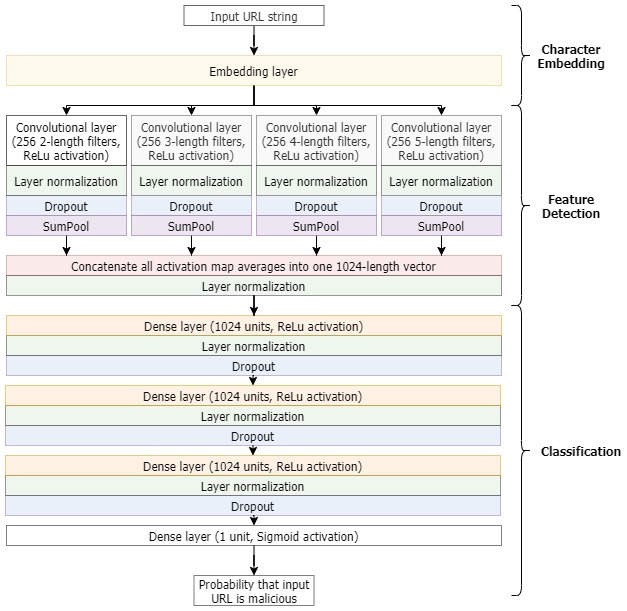
Figure 4 provides an overview of the model’s architecture.
Note: To speed up training and prevent overfitting, the model also has strategically placed dropout and layer-wise batch normalization layers. Dropout is equivalent to dropping some of the model’s little workers –neurons– every time. Neurons don’t know beforehand which ones are going to get dropped so all of them are forced to stay “sharp” in order for the model to stay on track with regards to keeping the loss function low. As for layer normalization, it provides a way for all layers to get input from preceding layers that is organized in a uniform way so as to make it easier for them to work with it.
So overall, this is how our CNN model works. With all of these parts, it is able to classify URLs as malicious or benign without needing to be spoon-fed any additional features. We have been able to verify its capabilities in comparison to other models that were created and optimized to solve the same task, and it is doing quite well.
Experimental results
Initially, we randomly sampled approximately 19,067,879 unique URLs from VirusTotal over a two-month period with the split shown in Table 1:
| URL types | Training | Testing |
| Benign | 7,211,705 | 9,718,748 |
| Malicious | 1,496,198 | 641,228 |
For comparison purposes, we implemented two baseline models:
- “N-gram”: A standard general feature n-gram extractor (n $\in [1,5]$)
- “Expert”: A model which uses manually extracted features including URL length, URL suffix tokens, and the domain name as done in [3].
The two models are built in such a way that they use different feature extraction methods (respectively as described above) but rely on the same classification neural network as our novel CNN architecture. In order to get the desired 1024-size list of numbers (our feature vector) that will be fed to the classifier, we use feature hashing to summarize all the extracted features (extracted according to the baseline model’s strategy).
Since this is a binary classification (classification across only two classes), and in real-life scenarios the occurrence of these classes is imbalanced (when browsing the web, think of the number of times you encounter benign web pages vs. malicious ones, it is absolutely not a 50-50 scenario), we cannot rely on metrics such as accuracy to reflect the performance of these models. This is why we evaluate the models based on the Receiver Operating Characteristic (ROC) curve between true positive and false positive rates. The true positive rate (TPR) captures the probability that a malicious URL gets correctly classified, whereas the false positive rate (FPR) represents the probability that a benign URL gets flagged as malicious. We want our TPR to be high –the model has a great nose for recognizing maliciousness, but at the same time we don’t want it to be erroneously flagging safe URLs as malicious (the FPR should be low). So we rely on the ROC curve to watch the tradeoff between these two metrics. The resulting ROC curves for all three models are presented below in Figure 5.
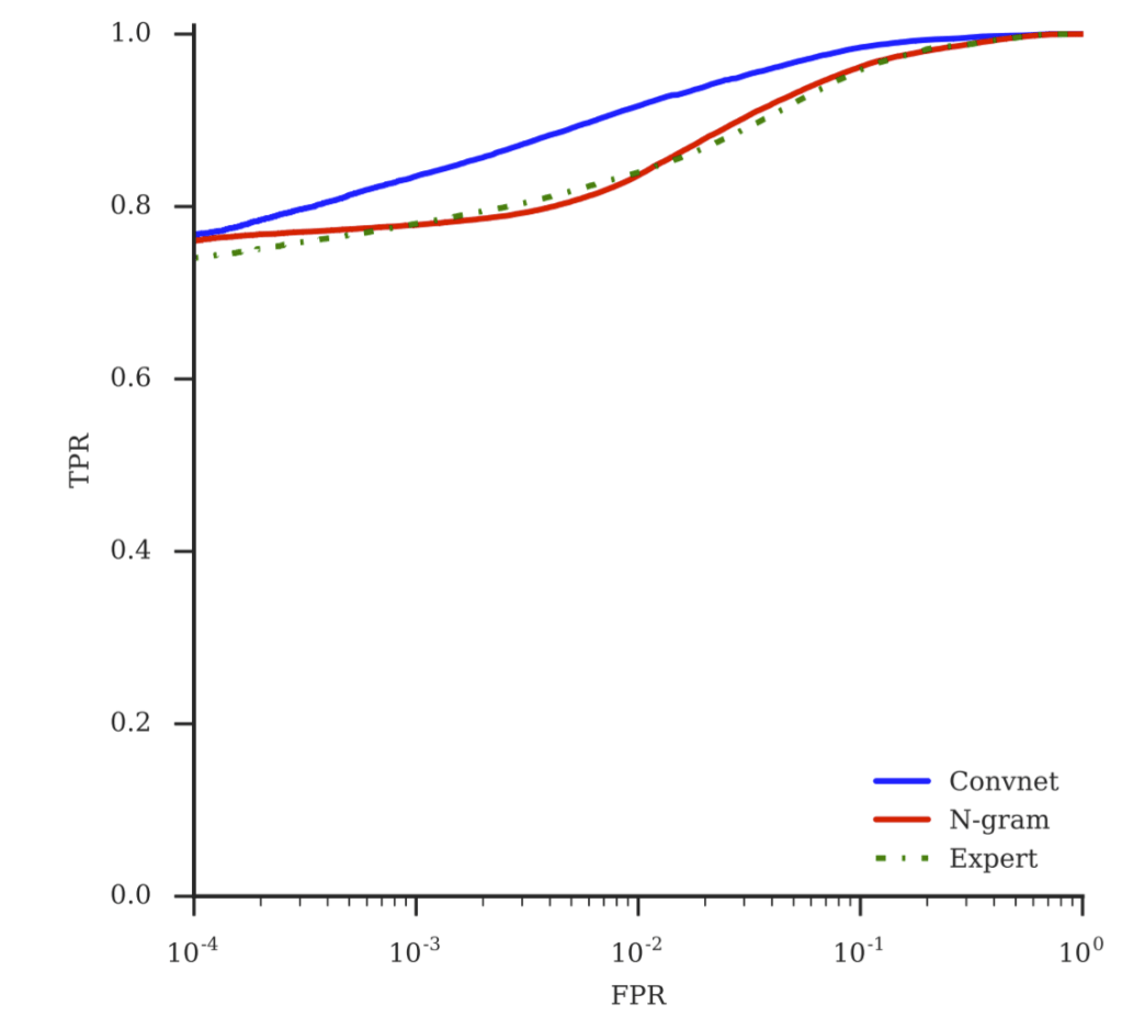
Table 2 captures more specific evaluation metrics for the three models. We give the TPR at different FPR values, as well as the area under curve (AUC) for the ROC.
Our ConvNet model clearly outperforms the other two model without using any hand-crafted features.
| Model | TPR at FPR=$10^{-4}$ | TPR at FPR=$10^{-3}$ | TPR at FPR=$10^{-2}$ | AUC |
| ConvNet | $\textbf{0.77}$ | $\textbf{0.84}$ | $\textbf{0.92}$ | $\textbf{0.993}$ |
| N-gram | $0.76$ | $0.78$ | $0.84$ | $0.985$ |
| Expert | $0.74$ | $0.78$ | $0.84$ | $0.985$ |
Conclusion
Developed back in 2017 by Sophos AI team members, this CNN approach to URL maliciousness detection was the first of its kind. Using embeddings and convolutional layers, the model is able to automatically extract relevant features from raw URL strings to solve the detection problem better than models that rely on additional manually extracted features.