
Previously in the ELI10 series, we went over our detector of malicious web content based on URLs: a lightweight deep learning approach which only requires the raw URL string to detect maliciousness. Continuing with malicious web resources, today we shed the light on another model; this one goes beyond mere URLs to take advantage of the full semantics of web content for the detection of maliciousness. It takes HTML documents as input and classifies them as either benign or malicious.
Introduction
The World Wide Web can be a dangerous place. Hackers are out to get your data, and one prominent weapon in their arsenal is malicious web content. By visiting the wrong web page, you might be opening Pandora’s box and compromising your computer’s security. Browsing malicious web content executes code whose objective can be to:
- Exploit browser software vulnerabilities to corrupt a user’s machine. E.g.: by discretely downloading malware in the background without asking you for your permission (aka. drive-by downloads).
- Exploit human fallibility by tricking users into providing sensitive information such as credit card numbers, login credentials, etc. This is generally referred to as phishing.
As such, a simple careless click on an infected page has the power to unleash pandemonium on your computer: hijacking your device for illegal ends, stealing your personal information, or just ruining your machine for the hell of it.
Scary stuff! And what’s even scarier is that it is very hard to differentiate between malicious and legitimate web content ourselves, especially with hackers working around the clock to outsmart the rest of us. Luckily, machine learning comes to the rescue. But before stacking neural network layers, we need to take a moment and consider what we are dealing with.
The challenges of detecting malicious HTML files
With HTML being the standard and most fundamental building block of every web page out there, we focus on HTML files as the representation of “web content”.
Okay, so are HTML files entirely and solely HTML?
Nope. That would be too easy. HTML files, in reality, can include HTML, CSS, as well as embedded JavaScript code. Alongside these different source code languages, the files may also contain embedded attack payloads, and natural language expressions within them, thus making them abundant in both semantics and syntax.
This richness of HTML files in structure and information makes the job of a maliciousness detector particularly hard:
- Different files can be of varying lengths, and can include different formats (HTML, CSS, JavaScript, English, etc.). A good detector should thus be able to learn a meaningful representation of the web content regardless of these differences.
- To go unnoticed, malicious code may come in very small snippets embedded within overall benign content. A good detector should be able to spot these malware needles in a haystack.
- Attackers also try to masquerade their malicious artifacts by using evasion techniques such as JavaScript obfuscation (where easy-to-read code is morphed into a deliberately obscure version) and text randomization. A good detector should see right through these evasion strategies.
- The detection of malicious web content should be performed without hindering a user’s browsing experience. A good detector must therefore act quickly on endpoints and firewalls.
Quite the list of challenges!
At Sophos, our AI team has been able to tick every item on this list with a carefully crafted classifier.
How does it work? That’s exactly what we will discuss next.
A high-level view of the web content classifier
At a high-level, given an input HTML document, our detector goes through three main steps:
- It breaks the input file into bite-size pieces (called tokens) based on a basic rule that we programmatically express using a simple, fast, 12-character regular expression.
- It then examines the resulting pieces at different hierarchical scales.
- Finally, it applies two dense neural networks over all the hierarchical levels and provides a maliciousness score which summarizes the detector’s verdict for the given input HTML file.
Let’s distill how these steps work to understand how they address the challenges we talked about earlier.
Step 1: Feature extraction process
Machine learning models like to deal with numbers. Consequently, we cannot just provide a raw HTML file as direct input to our detector, we first need to somehow translate it to representative numbers that encapsulate the meaning in the file so the model can tell whether it is unsafe or not. This is exactly what we set out to do in this step, which is coincidentally also how we tackle challenge #1 from the above list.
While reading this blogpost, you are weaving the meaning of this text word by word. Words are the text’s semantic units separated by whitespaces. But when it comes to a programming language, what would be the equivalent of a word? Especially with letters, special symbols, and numbers being all mashed up together. Still, given the programming language’s syntax, we can figure out some rules to separate a given code snippet into “words”. But, what about when one file incorporates a variety of programming languages as is the case in web content which can have HTML, CSS, and JavaScript all at once? Should we try to extensively process each one of them separately to eventually build an overall understanding of the entire file, or can we implement a fast format-agnostic strategy that would work regardless of the file’s constituent languages?
Sure enough, we went with the latter. The former alternative would involve processes like explicitly parsing, emulating, or symbolically executing the contents of HTML files, which are all legitimate ways of understanding what these files do, but these operations would be too computationally expensive (and would not help us overcome challenge #4).
Input tokenization
In order to break the HTML file into units which will get us closer to obtaining its numerical representation that a machine learning model can readily work with, we apply this simple 12-character regular expression (commonly called regex): ([ˆ\x00-\x7F]+|\w+). It might look like some arcane gibberish if you are unfamiliar with regexes, but it really is easy.
Mini regex crash course
Generally speaking, a regular expressions is just a sequence of characters used to capture a search pattern in a string. Let’s take ours for instance and examine its components:
(…): capture the string matched by the regex within them into a group.
[a-b]: matches a character within the specified range from a to b.
[^a-b]: matches a character NOT within the range from a to b.
\x00: refers to the ASCII table character at the hexadecimal position 0, which is the null character.
\x7F: refers to the ASCII table character DEL which is at the hexadecimal position 7F (equivalent to the number 127).
Note: At a fundamental level, computers only understand numbers. ASCII is a standard system that maps 128 symbols to numbers so computers can work with them. It is based on English alphabet letters (in both their lowercase and uppercase formats), punctuation, special symbols (e.g. $, +, =, etc.), digits, and some control codes (like ESC and DEL for example).
\w: is for “word characters” which may vary depending on the flavor of regex, but usually refers to ASCII letters, digits, and the underscore character.
+: to search for one or more of the pattern specified before it.
|: OR operand
With this in mind, let’s take another look at our regex:
- [ˆ\x00-\x7F]+ matches any one or more characters which are not in the ASCII table (from hexadecimal position 0 to 7F (7F is equivalent to the decimal 127)). It would for instance match the Arabic letter ﺱ.
- | OR
- \w+ matches any one or more word characters.
Tying it all together: the 12-character regex only captures strings of alphanumeric characters (and is not limited to just English letters) and those are will be our “words” or tokens from the input file that we will be working with.
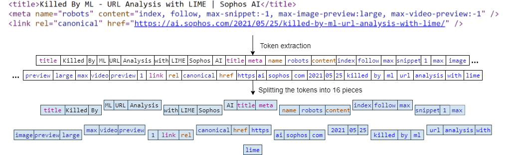
Consider the following HTML lines from one of our blogposts:

Applying our regex results in the following tokens:

TL;DR: The used regular expression essentially splits the input HTML document at non-alphanumeric characters thus breaking it into tokens regardless of the various formats it may contain.
So now that we have broken the file into pieces, we take the resulting sequence of tokens and proceed to splitting it into 16 sequential pieces of equal length (we define the length of the file $L$ as the total number of tokens). If $L$ is not divisible by 16, then all token chunks will have equal lengths except the last one which will subsequently have fewer tokens. This process is illustrated in figure 3 below.
Feature hashing
So far, we have broken the input document into tokens then we have sequentially grouped them into 16 equal-sized chunks. But we are still dealing with strings and have yet to translate them into meaningful numbers on which the detector can perform mathematical operations to be able to provide a classification decision. This is precisely when a neat trick comes into play: the “hashing trick” (also referred to as feature hashing). How does it work?
It relies on a hash function $h$. Such functions are extensively used in a myriad of fields in computer science. Think of $h$ as a factory that takes some raw material $x$ and turns it into a finished product $y$ (which is usually called hash value or simply hash) while making sure that its processing time is quite fast.
One thing that can happen with hash functions are hash collisions: this is when $h$ results in the same hash value for different $x$’s.
How does this relate to feature hashing? In our use case, the tokens we previously obtained are the “features” that our detector will rely on to predict whether their source HTML file is benign or malicious. We use a hash function $h$ that maps a feature $x$ to a hash value $y$ which is an integer between 0 and 1023 that represents its index in a 1,024-length vector: i.e. its position in a list of 1,024 numbers.
For each one of our 16 token chunks, we end up with a corresponding 1,024-length vector. Take one of those chunks: we initialize a vector of 1,024 zeros, Then each one of the tokens in that chunk is fed to $h$ which gives us its position in the corresponding vector, we then increment the value in the vector that is at that position. This way, we end up with 16 1,024-sized vectors which are precisely those representative numbers we were looking to get from the input file for the model to be able to investigate it with a machine learning model and make a maliciousness decision about it.
This feature extraction process also helps us in surpassing challenges #3 and #4. How?
A brief digression: Bag of words (BOW) representation
One common way of converting text into numbers to perform text classification is BOW representations. Given a set of texts that are to be classified, each unique word or token is added to a list referred to as the vocabulary and is assigned a unique integer (index), usually starting from 0. Then, for each text or file we would like our model to classify, we turn it into a vector that has the size of the vocabulary. For each token in that text, we perform a lookup in the vocabulary, get its corresponding index, and increment the vector entry at that index (at the beginning, the vector only has zeros), thereby turning the input text into a list of numbers the size of our vocabulary. That vector is a BOW representation. Pretty nice! Why didn’t we use this for the web content classification task on-hand?
For starters, BOW requires storing a vocabulary in memory which can be potentially huge. Feature hashing, on the other hand, does without such a requirement.
Additionally, malicious files can have some random strings and obfuscated code alongside benign legitimate content thrown in by attackers to fly under security radars and that were never-before seen in our data (out-of-vocabulary tokens). So even if we have an extensive vocabulary, it might not include these new strings which would go completely unnoticed and the resulting vector will not reflect their presence. So the model will not know about them and might misclassify this sample due to all the benign content that is contains. A potential solution would be to extend the vocabulary to include these new tokens, but then we would also need to retrain our classifier from scratch (since the input feature vector size changes too as it is precisely the vocabulary size) which can be time-consuming.
With feature hashing, due to the way we defined the hash function (that it necessarily maps to a specific range of integers, [0, 1,024] in our case), every token –even a never-before-seen one– is bound to increment a value in the resulting representation vector.
Note: We use a slightly modified version of feature hashing that also takes into consideration the token length. A code snippet can be found in our paper.
Now that we have worked out how to transform an HTML document into 16 1,024-length vectors where each one summarizes 1/16 of the original doc. How do we proceed with the actual classification?
Step 2: Neural network model
For solving the classification task, we use a neural network model. This model is actually made up of two logical components: an inspector model, followed by a main model. They are essentially two feed forward neural networks. The inspector model can be viewed as furthering the feature extraction exercise. It prepares a 1024-long vector that captures the meat of the HTML document and provides it to the main model which is responsible for making the final detection decision. In fact, these two components are optimized together, as one: the main model’s final decisions (given as probabilities that it computes for a bunch of HTML files) are compared to the true labels (whether a file truly is malicious or benign) using a loss function which captures how correct the model’s guesses were. The more incorrect the model’s predictions are, the higher the loss is. Throughout the training stage, the objective is to minimize said loss by adjusting the entire system (inspector and main model jointly).
Let’s look into the details of each one:
Inspector
The inspector model starts with an important step which enables our detector to conquer challenge #2. It takes our 16 vectors of length 1,024 and uses them to calculate hierarchical representations. The goal is to capture useful clues regarding the maliciousness of the overall file by inspecting it at various local spatial regions. This meticulous investigation helps in catching even small malicious snippets injected throughout an otherwise benign file.
Starting with the 16 vectors obtained earlier, the inspector averages the first 2 vectors (say $\mathbf{x}_1$ and $\mathbf{x}_2$) together entry by entry giving a new vector ($\mathbf{x}_{(1,2)}$), then goes on to the next 2 vectors ($\mathbf{x}_3$ and $\mathbf{x}_4$) and does the same thing, and repeats this process up until $\mathbf{x}_{(15,16)}$. This results in collapsing the original 16 vectors into 8 new ones. It then repeats the same process and collapses the 8 vectors into 4, then those 4 into 2, and finally those 2 into 1 as depicted in figure 4. This is equivalent to dividing the document into halves, quarters, eighths, and sixteenths.
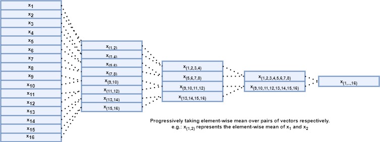
Eventually, we end up with 31 vectors (= the original 16 vectors + the (8+4+2+1) vectors resulting from the recursive averaging process explained above) representing a hierarchical representation of the original document by summarizing different parts of it at different scales. Then, the inspector applies the same set of fully connected (or dense) layers to each one of the 31 vectors. These are layers of 1,024 neurons (essentially units that perform a mathematical computation) each with ReLu activation (which gives the model the ability to solve complex problems like web content detection). They are called “fully connected” because each neuron in one layer is connected to every neuron in the other one. Their role is to look at each vector and find the most relevant patterns that would eventually help the main model figure out the maliciousness of the input file.
Apart from dense layers, the inspector also uses layer normalization and dropout. The former one outputs a better organized version of the input it got making it easier to digest for the layer on top of it. As for dropout, it is a mechanism that shuts off a percentage of neurons without prior indication as to which ones it will be. This forces the model to stay on its metaphorical toes: all neurons try and learn as best they can so even if some of them are “dropped”, the remaining ones can still manage to find useful clues and help the overall model make correct decisions. A visualization of the inspector model is shown in figure 5.
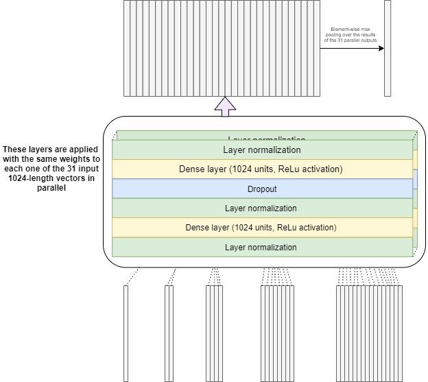
By applying the same neural network model to each one of the 31 vectors in parallel, we obtain 31 1,024-length output vectors. To summarize them into a unique 1,024 vector that would hold the most important information that the inspector found, we just take the maximum for each one of the 1,024 output neurons across all 31 outputs.
Okay, so now we have ONE 1,024 length vector that represents everything we have found out so far about the input document. It is thus given to the main model as input who will provide us with a decision: one number expressing this entire system’s conclusion about how probable it is that the input file is a malicious one.
Main model
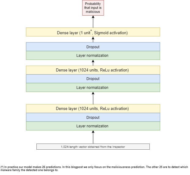
We can now get to the actual classification process with the main model. It has two sequential fully connected blocks. Each block has a dense layer of 1,024 neurons preceded by layer normalization and dropout. We also use layer normalization and dropout on top of the second block before our last dense layer which only has one unit and uses sigmoid activation which is a mathematical function that finally gives us the Holy Grail: the maliciousness prediction (the probability that the input HTML file is malicious).
Figure 6 presents an overview of the main model’s architecture.
As mentioned earlier, the inspector and main models are trained and optimized together. The loss function on which this optimization relies is binary cross-entropy.
Experimental results
Using an experimental dataset of labeled HTML files collected from VirusTotal (VT) over a 10-month period. This dataset is split into training and testing sets based on the time a web content file was first reported on VT.
To see how our model fares in comparison to other alternative approach, we use two baseline models. The input to these two models consists of a feature vector of length 16,284. This vector is constructed by taking the tokens extracted for our hierarchical model and applying feature hashing to obtain the 16,284-length list of feature values. This is done in order to have a feature vector of the same dimensionality as the 16×1,024 input given to our hierarchical model. The two baseline models used for comparison are:
- XGBoost-BoT: An XGBoost model.
- FF-BoT: A feed-forward network which represents a deep-learning BoW baseline to compare our model to.
Note: All neural network approaches used in our experiments, including our model, are optimized using the Adam method and trained using balanced (50-50 benign and legitimate files) batches of 64 input files every time. We also use the “early stopping” strategy where we put an end to training as soon as the model’s performance on the validation set starts to stagnate for a chosen number of training iterations.
As the web-content maliciousness detection task we are trying to solve is essentially an imbalanced (there are much more binary files than maliciousness ones in real-life) binary (is the input HTML file legitimate or malicious?), we evaluate the models based on their ROC curves and compare them accordingly. Figure 7 shows the resulting curves capturing the performance of our hierarchical model in comparison to the two baseline approaches.
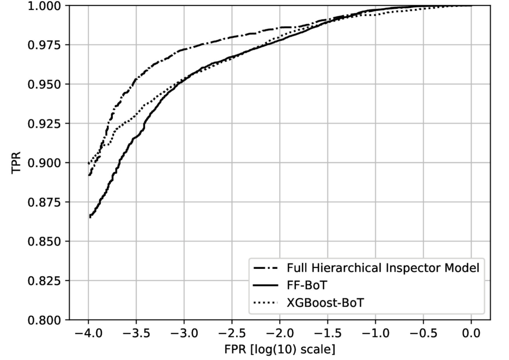
Our hierarchical model is far superior to the other two baseline models. It was able to achieve an impressive 97.2% detection rate (i.e. it detected 97.2% of all malicious HTML files) at a 0.1% false positive rate (i.e. while only misclassifying a mere 0.1% benign files as malicious) while ticking all the items on our list of challenges posed by the problem of web content classification. In comparison, at the same false positive rate, XGBoost-BoT has a detection rate of 95.4% while FF-BoT achieves 95.2%.
Additionally, the FF-BoT neural network baseline uses around 20 million parameters, compared to our inspector-main model which only requires approximately 4 million parameters and still outperforms its flat feed-forward baseline counterpart. This is quite revealing of the ability of our proposed solution to skillfully capture meaningful numerical representations of web content files. With its efficient parameter sharing scheme (the inspector model relies on the same set of parameters to examine the input at a variety of spatial regions), it keeps the number of needed parameters low while also achieving impressive results.
Conclusion:
By using what we know about web content attacks and baking it into a detection pipeline, our team has been able to produce a powerful maliciousness detector acting on HTML files. This model has seen the light of day back in 2018 and is still going strong in its detection performance. For further details, please check out the team’s published paper.